Your TTS Model Can Speak. Why Does It Still Sound Wrong?

Same Model. Just 10 Hours of Fine-Tuning. Hear the Difference.

Before Fine-Tuning | After Fine-Tuning

Same text. Same reference audio. Same inference settings.

1. Introduction: Why TTS Still Needs Post-Training

I've run into a few recurring problems while training TTS models.

The beginning of a generated clip can be unstable. Longer sentences, unusual phrasing, and unfamiliar words sometimes cause mispronunciations, skipped words, or repetitions. Even with the same text and reference audio, different samples can sound surprisingly different. One might be smooth and natural, while another has awkward pauses, odd intonation, or shifts in voice quality.

Of course, variation isn't always a bad thing. We want speech to sound expressive and natural. We also want the model to read the text correctly and preserve the speaker's identity.

Model architectures keep improving, and pre-training datasets keep growing, but these problems haven't disappeared. Not every issue needs another round of training, either. Text normalization, alignment, and sampling strategies can all affect the output.

That's what got me interested in TTS post-training. Given a model that can already generate speech, can we use more targeted training to make it perform the way we want?

1.1 How Does TTS Generate Speech?

Before getting into post-training, here's a quick look at two common approaches to speech generation.

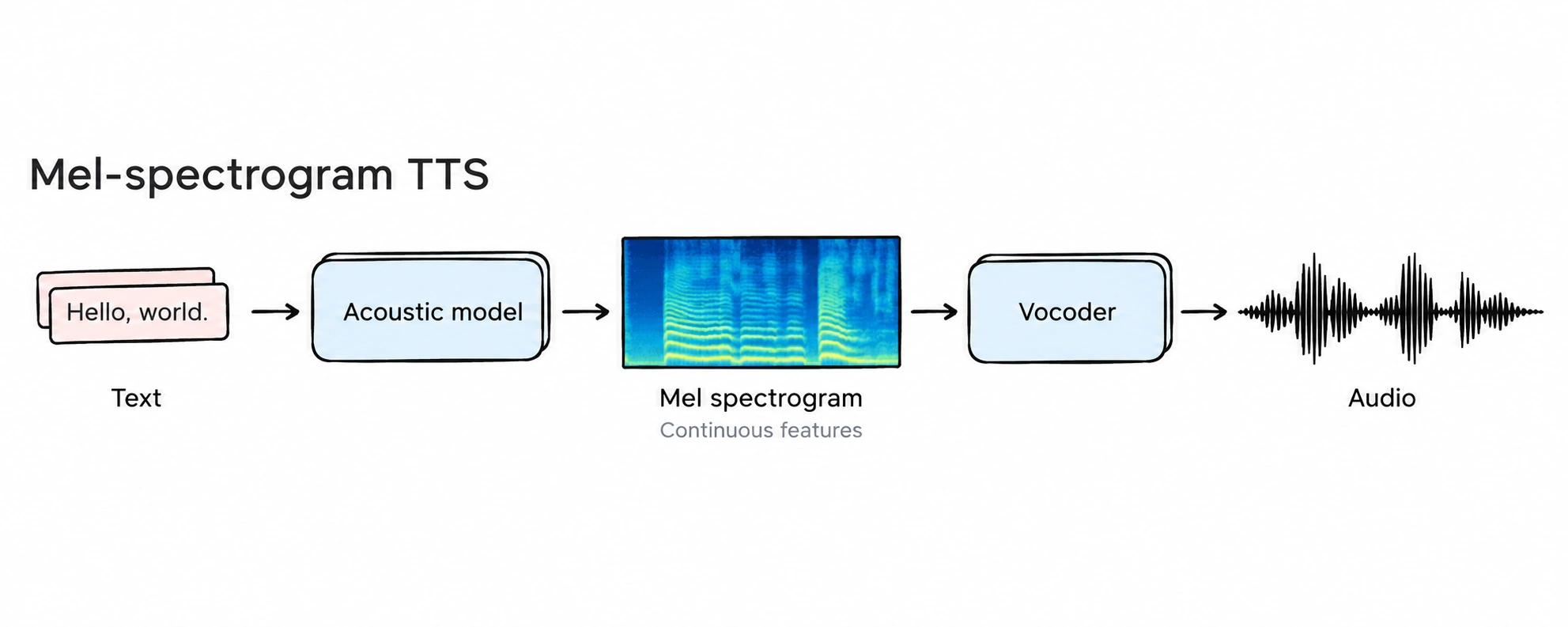
In a classic neural TTS pipeline, an acoustic model predicts a Mel spectrogram from text, and a vocoder turns those acoustic features into a waveform.

Mel spectrogram: A time-frequency representation of audio, with its frequency scale designed to roughly reflect how we perceive pitch.
Vocoder: A model that synthesizes an audio waveform from acoustic features such as a Mel spectrogram.

Our work focuses on language model-based TTS. In one common autoregressive setup, a neural audio codec encodes speech into discrete audio tokens. A Transformer then learns to predict those tokens from text and other conditioning inputs, and the codec decoder converts the generated tokens back into audio.

Neural audio codec: A model that compresses audio into a compact representation and reconstructs audio from it. Some codecs use discrete tokens that can be modeled by a language model.

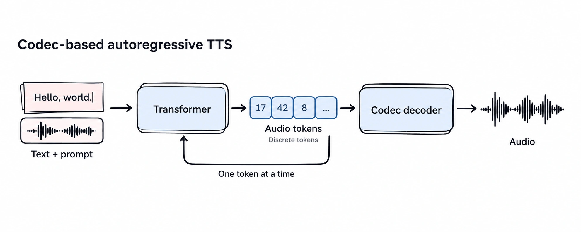
Mel-spectrogram TTS: text to acoustic features, then a waveform.

Codec-based autoregressive TTS: predict audio tokens, then decode them into speech.

The autoregressive part is similar to next-token prediction in a language model, except the tokens represent speech rather than text.

These are just two representative approaches. Modern TTS also includes diffusion and flow-matching methods. I won't try to cover every architecture here. The rest of this post focuses on post-training for language model-based TTS.

1.2 From Pre-Training to Post-Training

Pre-training teaches a model the relationship between text and speech, including pronunciation, speaker characteristics, and different ways of speaking, using large amounts of data.

But knowing how to generate speech doesn't mean a model can reliably do everything we need. It might still struggle with complex sentences or drift away from a target speaker's voice and delivery.

Post-training gives us another option. We can use more targeted data and training objectives to move the model toward the results we want, while trying to preserve the capabilities it already has.

A natural place to start is supervised fine-tuning (SFT). I want to look at what supervised data actually teaches the model, and why preference optimization may still be useful afterward.

2. Supervised Fine-Tuning (SFT)

Supervised fine-tuning continues training an existing model on data selected for a particular goal, such as pronunciation, speaker identity, or speaking style.

2.1 The SFT Objective

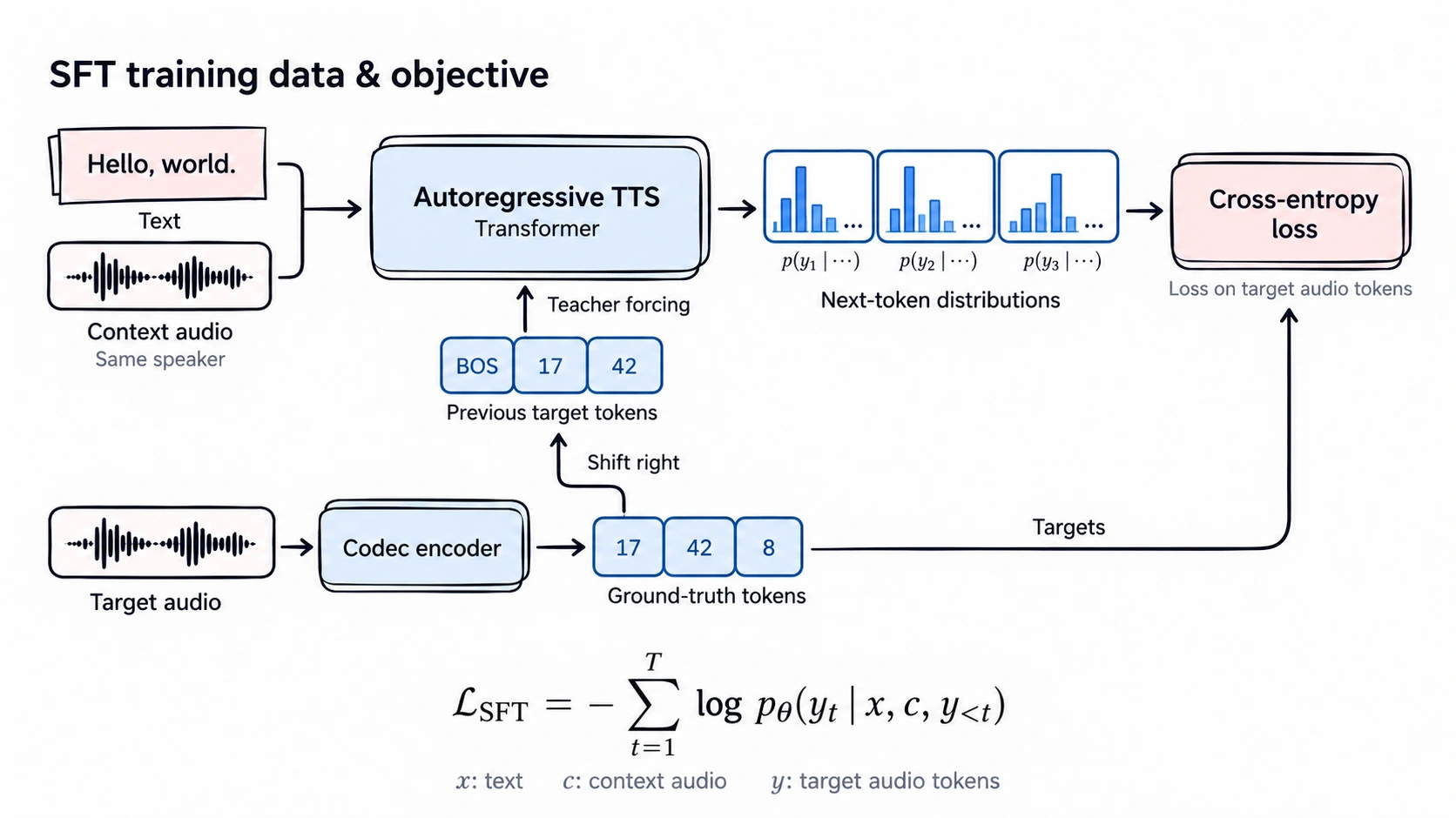
For autoregressive language model-based TTS, a common approach is to use cross-entropy loss to predict the next audio token from the text, reference audio, and preceding tokens.

The simplified objective is:

\mathcal{L}_{\mathrm{SFT}}(\theta)=-\mathbb{E}_{(x,y)\sim\mathcal{D}}\left[\sum_{t=1}^{T}\log p_{\theta}(y_t\mid y_{<t},x)\right]

Here, $x$ represents the conditioning inputs, such as text and reference audio; $y$ is the target sequence of audio tokens produced by a codec; and $\theta$ denotes the model parameters.

During training, we typically use teacher forcing: the model receives the ground-truth previous tokens when predicting the next one. Minimizing the negative log-likelihood (NLL) increases the probability the model assigns to the target audio sequence.

This is a form of maximum likelihood estimation (MLE). The equation describes a simplified single-stream autoregressive model. Real systems may use multiple codebooks and additional auxiliary losses.

2.2 Training Data: Quality Before Sheer Volume

Beyond the objective itself, I think data quality deserves just as much attention.

For reference-conditioned TTS, a training example often has three parts:

Text: The transcript of the target speech.
Context audio: A reference clip that provides information about the speaker's voice.
Target audio: The actual recording the model is trained to predict.

The context and target clips typically come from the same speaker, though they can contain different utterances.

SFT training data and objective: text and context audio condition next-token prediction, supervised by target audio tokens.

First, the supervision has to be reliable. The text should match the recording, speaker labels should be consistent, and the audio should be free of serious noise or distortion.

LibriTTS-R is a useful example. Its authors used speech restoration to improve the recording quality of a TTS dataset and reported improvements in downstream TTS evaluations.

But clean audio isn't automatically good training data. Pronunciation, rhythm, pauses, intonation, and emotional expression matter too. We want the model to learn how speech sounds in different contexts, not just how to pronounce the words.

That doesn't mean every clip needs strong emotion. Calm, natural speech matters just as much. For me, the goal is to balance reliable supervision with enough variation in the speaking styles we actually want the model to learn, rather than simply collecting more hours.

2.3 What SFT Can and Can't Do

SFT can help a model adapt to a speaker, pronunciation patterns, and speaking style. But its objective is still to make the model more likely to generate the target recordings in its training data.

A lower training loss doesn't necessarily mean listeners will prefer the output.

Given the same text, a model might produce several intelligible samples that differ in pacing, naturalness, or speaker consistency. Standard SFT doesn't directly use the relative quality of those samples as a training signal.

That led me to a different question: what if, instead of only showing the model a good example, we could also tell it which of its own outputs we prefer?

That's where preference alignment comes in.

3. Preference Alignment: Direct Preference Optimization (DPO)

SFT teaches the model to reproduce target speech, but it doesn't explicitly compare the quality of different outputs. Direct Preference Optimization (DPO) takes a different approach. It uses pairs of preferred and less-preferred outputs to change how likely the model is to generate each one.

3.1 How Do We Define Speech Quality?

DPO doesn't decide what good speech sounds like on its own. We need a way to label one candidate as chosen and another as rejected.

Drawing on Koel-TTS and Preference Alignment Improves Language Model-Based TTS, three practical automated measures are:

Dimension	Metric	What it measures
Text accuracy	CER / WER (lower is better)	An ASR model transcribes the generated audio, then we compare it with the input text.
Speaker similarity	Speaker similarity (higher is better)	A speaker verification model compares embeddings from the generated and reference audio.
Perceptual quality	Proxy MOS (higher is better)	A model such as UTMOS predicts a perceptual quality score.

Different metrics can disagree. Koel-TTS uses Pareto ranking, while Preference Alignment explores combining candidates' ranks across metrics. Both are ways to construct preference labels, not requirements of DPO itself.

These aren't the only qualities that matter. They're useful largely because we can evaluate them automatically at scale. Emotion, prosody, and whether a delivery fits the context are harder to capture reliably. Listening tests and human preference labels still have a role to play. As evaluation methods improve, I'd like to look beyond these three metrics.

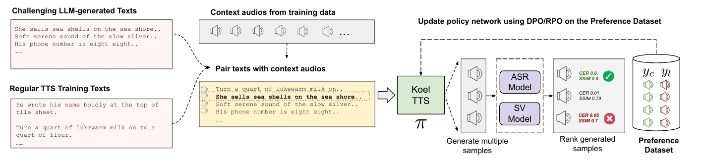
Koel-TTS preference alignment: generate, evaluate, and rank speech candidates to construct preference pairs.

Figure source: Hussain et al., Koel-TTS: Enhancing LLM based Speech Generation with Preference Alignment and Classifier Free Guidance, Figure 2, EMNLP 2025, CC BY 4.0.

3.2 The DPO Objective

For the same text and reference audio, we can use these metrics to select a preferred sample and a less-preferred one. Each preference example has the form $(x,y^{+},y^{-})$ , where $x$ is the conditioning input and $y^{+}$ and $y^{-}$ are the audio-token sequences for the chosen and rejected samples.

The standard DPO loss is:

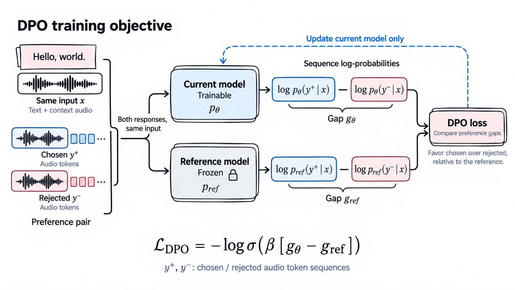
\mathcal{L}_{\mathrm{DPO}}(\theta)=-\mathbb{E}_{(x,y^+,y^-)\sim\mathcal{D}}\left[\log\sigma\left(\beta\left[\log\frac{\pi_\theta(y^+\mid x)}{\pi_{\mathrm{ref}}(y^+\mid x)}-\log\frac{\pi_\theta(y^-\mid x)}{\pi_{\mathrm{ref}}(y^-\mid x)}\right]\right)\right]

DPO training objective: compare chosen and rejected sequences under the current and frozen reference models; update only the current model.

The formula comes down to two comparisons.

First, there's the current model versus the reference model. The current model is updated during training. The reference model stays fixed, giving us a baseline for changes in log-probability.

Second, there's chosen versus rejected. We want the current model to favor the chosen output more strongly relative to the rejected one than the reference model does.

So DPO isn't simply about increasing the absolute probability of the chosen sample. It optimizes the relative preference, without needing a separately trained reward model in the optimization loop.

3.3 Key Parameters and Practical Details

Reference model: This is typically a frozen copy of the model at the start of DPO training. Only the current model is updated. An additional SFT stage is not a strict prerequisite.

Beta ( $\beta$ ): This controls the DPO objective. In the original KL-regularized formulation, a larger beta corresponds to a stronger penalty for moving away from the reference policy. It isn't the learning rate or a weight assigned to CER or speaker similarity. Preference Alignment found $\beta=0.01$ worked best in its experiments, but that value isn't universal.

Sequence log-probability: For autoregressive TTS, we sum token log-probabilities across the generated audio sequence. DPO needs this value for both the chosen and rejected samples, under both the current and reference models.

Length normalization: Dividing the summed log-probability by the token count changes the scale of the comparison. Preference Alignment tested this and ultimately kept the non-normalized version because it did not improve on its best configuration.

3.4 Reward-Aware Preference Optimization (RPO)

Not all preference pairs are equally clear-cut. Sometimes the chosen and rejected samples sound almost identical. Other times the difference is obvious.

Standard DPO uses which sample is preferred, not the numerical gap between their scores. Reward-Aware Preference Optimization (RPO) also uses that gap, aiming to make the model's implicit preference strength reflect the reward difference.

A compact form of the objective is:

\mathcal{L}_{\mathrm{RPO}}=\mathbb{E}_{\mathcal{D}}\left[\mathbb{D}\left(\beta m_\theta\parallel\eta\Delta r\right)\right]

Here, $m_\theta$ is the log-probability preference margin from DPO, $\Delta r$ is the reward gap between the chosen and rejected samples, and $\eta$ controls its scale. In the Koel-TTS formulation, $\mathbb{D}$ measures the KL divergence between the corresponding preference probabilities after applying a sigmoid.

The idea is to avoid treating a tiny quality difference exactly like a large one. But that also means the reward magnitudes need to be meaningful. RPO isn't necessarily better than DPO, so we're keeping DPO as our main approach and treating RPO as something to explore later.

4. Preference Data Construction

Once we've settled on a preference objective, the next question is practical: which inputs should we generate samples for, and how do we turn those samples into reliable preference pairs?

4.1 A Difficult Text Dataset Built from Failure Cases

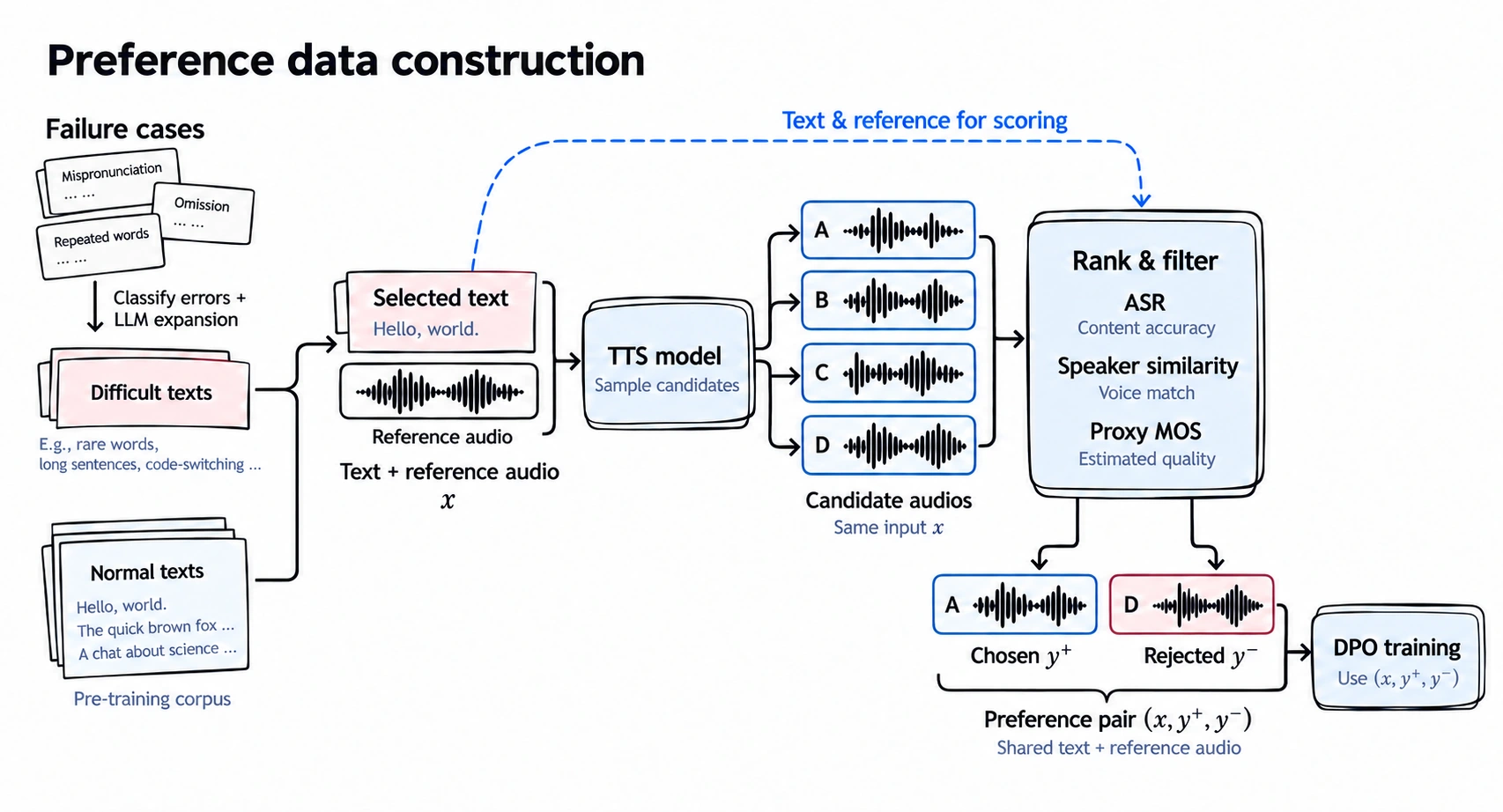
While training and testing TTS models, we kept seeing the same kinds of mistakes. Unusual sentence structures, rare words, and certain text patterns could trigger mispronunciations, missing words, or repetitions.

And difficult text doesn't necessarily mean long text. Repeated words, number sequences, similar-sounding words, and even short sentences can be surprisingly hard for a TTS model.

Instead of just adding more random text, we decided to build a dataset around these failure cases. We first collected examples where the model struggled, grouped them by error type, and then used an LLM to generate more examples in each category.

In our earlier experiments, we used Qwen3.5-27B to generate an initial set of about 8,000 difficult texts. We wrote prompts for different error categories, then checked, deduplicated, and filtered the results to keep useful examples.

A sentence that looks tricky to us isn't necessarily difficult for the model, though. We still need to run these texts through the base model and check whether they expose the failure modes we're trying to study.

We also mix in normal text drawn from our pre-training corpus, so the preference dataset doesn't focus exclusively on a small set of edge cases.

4.2 From Input Text to Preference Pairs

With the text dataset ready, we can use the TTS model to generate candidates.

For each text and reference-audio pair, we keep the conditioning inputs and sampling settings fixed, then draw multiple samples. We evaluate them using the ASR, speaker similarity, and predicted perceptual quality metrics introduced earlier, and rank the candidates.

From there, we choose a relatively strong sample as chosen and a weaker one as rejected, producing the pairs used for DPO training.

One detail matters here: the chosen sample doesn't have to be a human recording.

In Preference Alignment Improves Language Model-Based TTS, pairing a ground-truth recording with a model-generated rejected sample performed worse than selecting both sides of the pair from model-generated candidates. The authors suggest that distribution differences in discrete audio-token space may make the ground-truth-versus-generated comparison too easy, without teaching the model enough about quality differences among its own outputs.

For that reason, we prefer to construct both chosen and rejected samples from the same model's generations rather than assuming a human recording is always the best positive example.

Even then, the top-ranked candidate isn't guaranteed to be good. If the samples are too similar, or the metrics disagree too strongly, we may need to discard the pair rather than force a preference label.

The resulting dataset combines regular and difficult inputs with model-generated preference pairs. Whether it improves performance on challenging text is something we'll need to check on a separate held-out test set.

Preference data construction: combine difficult and regular texts, generate candidates, then rank and filter chosen/rejected pairs.

5. Classifier-Free Guidance (CFG)

Besides DPO, we also looked at classifier-free guidance (CFG) as used in Koel-TTS. During training, Koel-TTS randomly drops the text and reference-audio conditioning inputs with a probability of 10%. This condition dropout teaches the same model to make both conditional and unconditional predictions, which can later be combined to strengthen conditioning at inference time.

Only the conditioning inputs are dropped, not the target audio used for supervision. Koel-TTS introduces this capability during base-model training, and CFG is not a required part of DPO.

At inference time, the two sets of logits are combined as follows:

\ell_{\mathrm{CFG}}=\gamma\ell_c+(1-\gamma)\ell_u

Here, $\ell_c$ and $\ell_u$ are the conditional and unconditional logits, and $\gamma$ is the CFG scale. Setting $\gamma=1$ gives ordinary conditional generation. Values above 1 increase the influence of the conditioning inputs.

Koel-TTS reports improvements in text accuracy and speaker similarity with CFG, including when it is combined with DPO. But a higher scale isn't automatically better for overall speech quality. The right value has to be tested for the model in question.

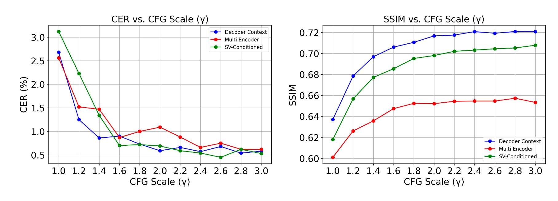
Koel-TTS Figure 5: character error rate and speaker similarity across classifier-free guidance scales.

Figure source: Hussain et al., Koel-TTS: Enhancing LLM based Speech Generation with Preference Alignment and Classifier Free Guidance, Figure 5, EMNLP 2025, CC BY 4.0.

6. Discussion & Future Work

This post covers the approach we've been exploring, from SFT and preference alignment through DPO and CFG.

We're still running experiments and pulling together the inference and evaluation results, so I don't have a complete experimental record to share yet. For now, I wanted to write down how we arrived at these choices. I'll add the results and anything new we learn as the experiments progress.

There are also a few open problems I keep coming back to.

The first is evaluation. CER, speaker similarity, and Proxy MOS tell us useful things, but they don't capture everything that makes speech sound right. Emotion, prosody, and whether a delivery fits the context remain hard to evaluate automatically.

The second is preference-data quality. DPO learns from the labels we give it. If those labels reflect biases in the automatic metrics, better scores won't necessarily translate into a better listening experience.

I'd like to see more fine-grained human annotations, better multidimensional speech-quality models, and listening evaluations that help close that gap.

For me, this post is a record of learning, reading the research, and putting ideas into practice. We take what seems useful from previous work, adapt it to the models we're training, and test whether it actually helps.

We're still training and testing new models and methods. As we get more results, I'll update the post with what worked, what didn't, and anything that changes my mind along the way.

In the end, the actual speech is what matters. That's where these ideas have to prove themselves.